Effect of the smoothing factor

import pymultipleis as pym

import numpy as onp
import jax.numpy as jnp

# Load the file containing the frequencies
F_her = jnp.asarray(onp.load('../../../data/her_50/freq_50.npy'), dtype=jnp.float64)
# Load the file containing the admittances (a set of 50 spectra)
Y_her = jnp.asarray(onp.load('../../../data/her_50/Y_50.npy'))

WARNING:absl:No GPU/TPU found, falling back to CPU. (Set TF_CPP_MIN_LOG_LEVEL=0 and rerun for more info.)

# Define model
def her(p, f):
    w = 2*jnp.pi*f
    s = 1j * w
    Rs = p[0]
    Qh = p[1]
    nh = p[2]
    Rad = p[3]
    Cad= p[4]
    nad= p[5]
    Rct= p[6]
    Wct=p[7]
    Zw = Wct/jnp.sqrt(w) * (1-1j)
    Zct   = Rad + Zw
    Yca=(((s**nad)*Cad) + Rct**-1)
    Z1=(Yca**-1 +Zct)
    Y1=(Z1**-1)
    Ydl= ((s**nh)*Qh)
    Z = (Rs + (Ydl + Y1)**-1)
    Y = 1/Z
    return jnp.concatenate((Y.real, Y.imag), axis = 0)

p0 = jnp.asarray([4.72774187e+02, 9.70785283e-07, 6.51261304e-01,
             1.04825669e+03, 7.27786796e-07, 8.33955442e-01,
             5.98926963e+04, 2.03231984e+04], dtype = jnp.float64)

bounds = [[1e-3,  1e6], [1e-9, 1e-1], [1e-1, 1], [1e-5, 1e8], [1e-9,  1e-1], [1e-1, 1], [1e-5,  1e8], [1e-5,  1e8]]
smf_modulus = jnp.full((len(p0),),1.0)

1. Fit simultaneous without a smoothing factor of zero

eis_her = pym.Multieis(p0, F_her, Y_her, bounds, smf_modulus, her, weight= 'modulus', immittance='admittance')
popt, perr, chisqr, chitot, AIC = eis_her.fit_simultaneous_zero()
print(chitot)
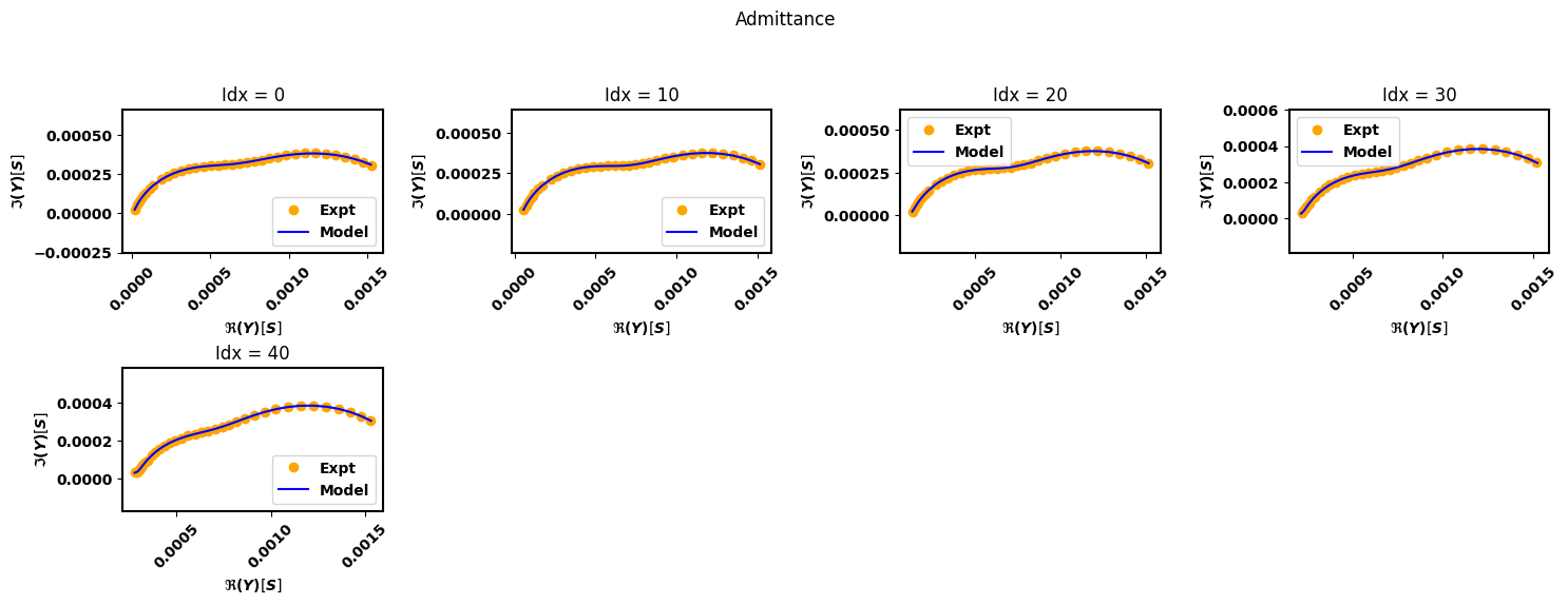
eis_her.plot_nyquist(10)
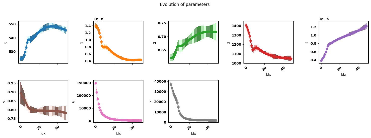
eis_her.plot_params()
eis_her.plot_params(show_errorbar=True)

Using initial

Optimization complete
total time is 0:00:14.503258 0.0005054471650576946

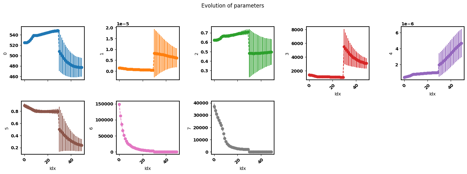
2. Fit sequential (i.e. fit individual spectra using least squares)

eis_her = pym.Multieis(p0, F_her, Y_her, bounds, smf_modulus, her, weight= 'modulus', immittance='admittance')
popt, perr, chisqr, chitot, AIC = eis_her.fit_sequential()
eis_her.plot_nyquist(10)
eis_her.plot_params()
eis_her.plot_params(show_errorbar=True)

Using initial
fitting spectra 0
fitting spectra 10
fitting spectra 20
fitting spectra 30
fitting spectra 40

Optimization complete
total time is 0:01:03.492508

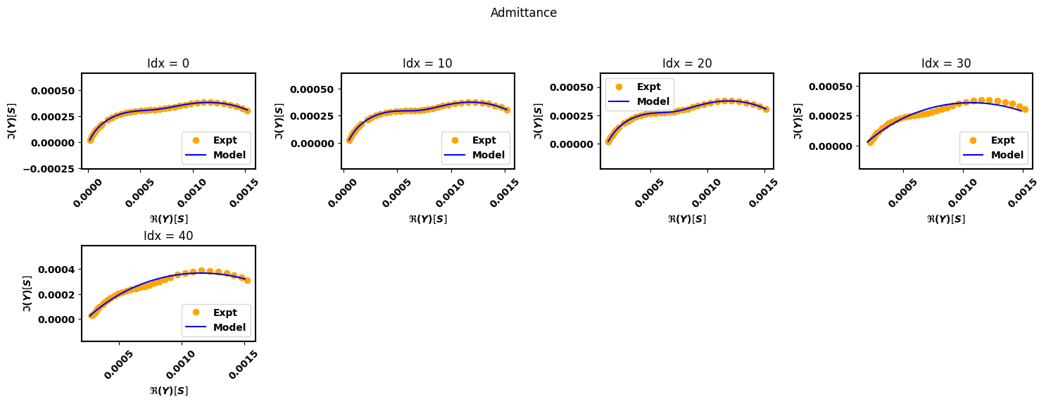
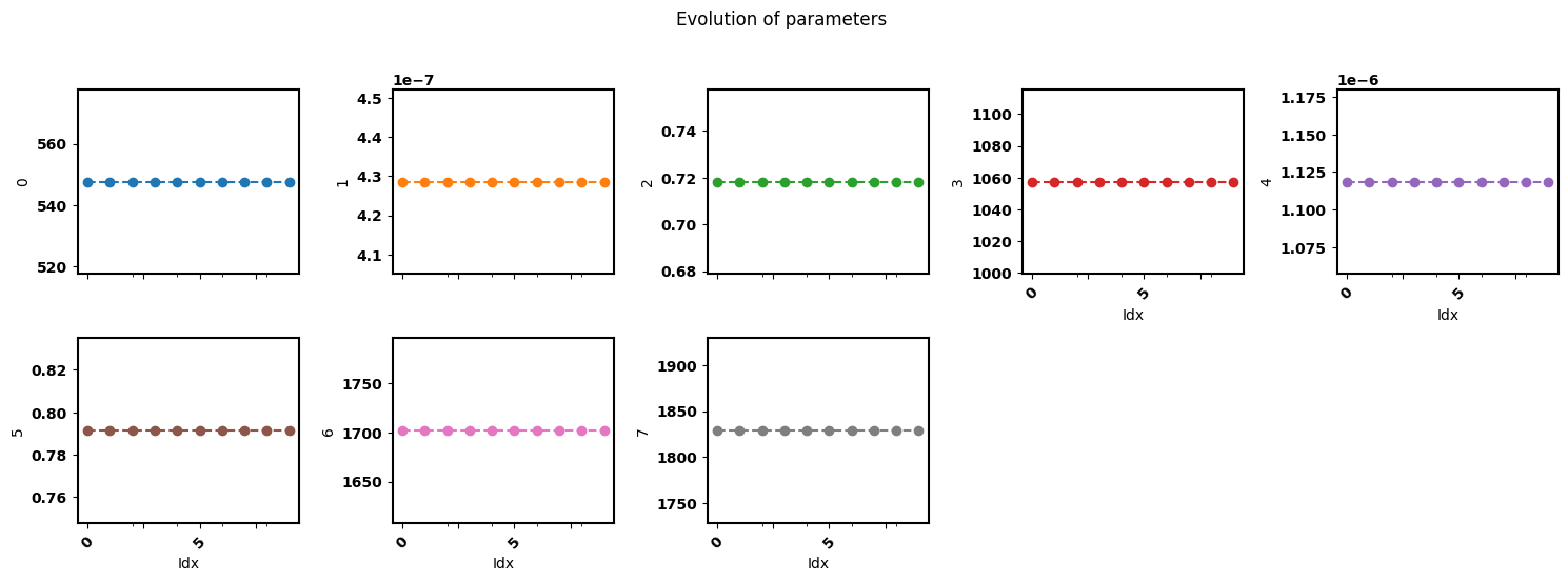
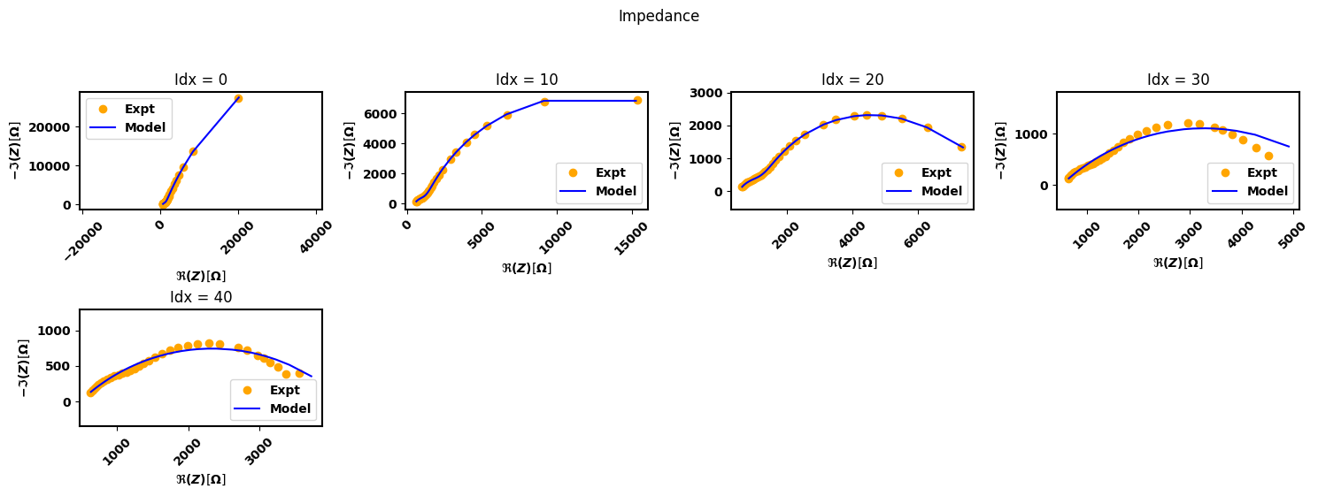
3. Use a smoothing factor to obtain reasonable initial values before setting the smoothing factor to zero

eis_her = pym.Multieis(p0, F_her, Y_her, bounds, smf_modulus, her, weight= 'modulus', immittance='admittance')

chi=eis_her.compute_total_obj(eis_her.convert_to_internal(p0), eis_her.F, eis_her.Z, eis_her.Zerr_Re, eis_her.Zerr_Im, eis_her.lb_vec, eis_her.ub_vec, eis_her.smf)

eis_her = pym.Multieis(p0, F_her, Y_her, bounds, smf_modulus, her, weight= 'modulus', immittance='admittance')
popt, perr, chisqr, chitot, AIC = eis_her.fit_simultaneous(method='L-BFGS-B')
print(chisqr)
popt, perr, chisqr, chitot, AIC = eis_her.fit_simultaneous_zero()
eis_her.plot_nyquist(10)
eis_her.plot_params()
eis_her.plot_params(show_errorbar=True)

Using initial

Optimization complete
total time is 0:00:11.225109 4.669901034830563e-06

Using prefit

Optimization complete
total time is 0:00:05.984875

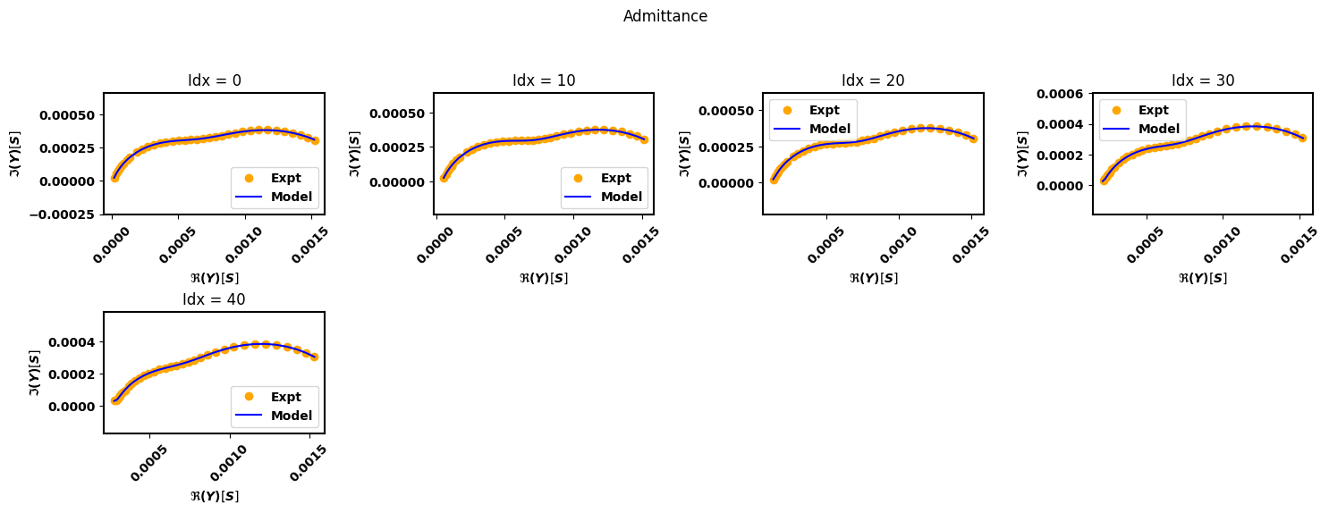
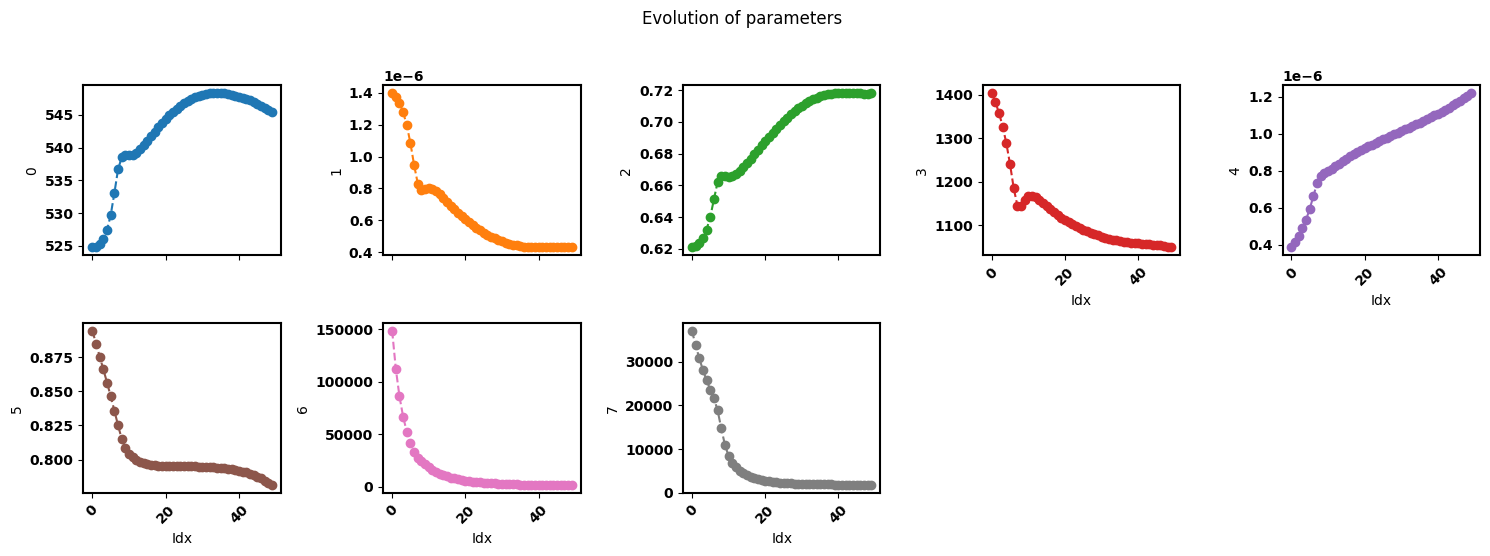
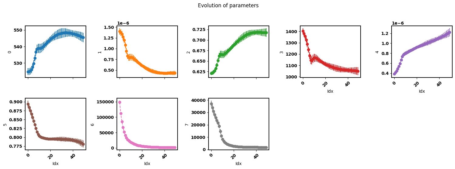
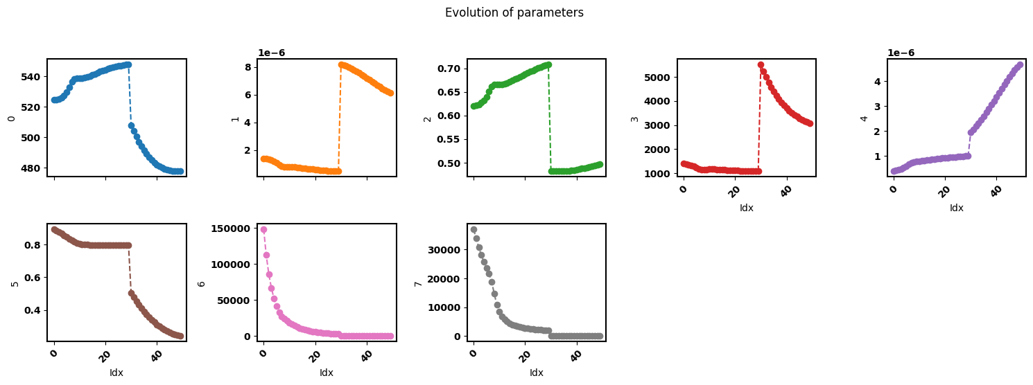
4. Use a smoothing factor to obtain reasonable initial values before fitting each spectra individually

eis_her_simultaneous = pym.Multieis(p0, F_her, Y_her, bounds, smf_modulus, her, weight= 'modulus', immittance='admittance')
popt, perr, chisqr, chitot, AIC = eis_her.fit_simultaneous()
popt, perr, chisqr, chitot, AIC = eis_her.fit_sequential()
eis_her.plot_nyquist(10)
eis_her.plot_params()
eis_her.plot_params(show_errorbar=True)

Using prefit

Optimization complete
total time is 0:00:04.744852
Using prefit
fitting spectra 0
fitting spectra 10
fitting spectra 20
fitting spectra 30
fitting spectra 40

Optimization complete
total time is 0:00:56.096820

Repeating a single spectra (What to do when you have a single spectra to fit)

Y_her_single_spectra = Y_her[:, 41]
Y_her_single_spectra.shape
# torch.Size([35])

(35,)

Y_her_repeated = jnp.tile(Y_her_single_spectra[:,None], (1, 10))
Y_her_repeated.shape
# torch.Size([35, 10])

(35, 10)

smf = jnp.full((len(p0),), jnp.inf)
eis_her = pym.Multieis(p0, F_her, Y_her_repeated, bounds, smf, her, weight= 'modulus', immittance='admittance')
# popt, perr, chisqr, chitot, AIC = eis_her.fit_simultaneous()
popt, perr, chisqr, chitot, AIC = eis_her.fit_stochastic()
popt, perr, chisqr, chitot, AIC = eis_her.fit_sequential()
eis_her.plot_nyquist(2)
eis_her.plot_params()
eis_her.plot_params(show_errorbar=True)

Using initial
0: loss=9.370e-02
10000: loss=4.670e-04
20000: loss=3.162e-06
30000: loss=3.171e-06
40000: loss=3.162e-06
50000: loss=3.162e-06
60000: loss=3.162e-06
70000: loss=3.162e-06
80000: loss=3.162e-06
90000: loss=3.162e-06
Optimization complete
total time is 0:00:52.636309
Using prefit
fitting spectra 0

Optimization complete
total time is 0:00:11.123443