Getting started
[1]:
import pymultipleis as pym
[2]:
import numpy as onp
import jax.numpy as jnp
[3]:
# Load the file containing the frequencies
F = jnp.asarray(onp.load('../../../data/redox_exp_50/freq_50.npy'))
# Load the file containing the admittances (a set of 50 spectra)
Y = jnp.asarray(onp.load('../../../data/redox_exp_50/Y_50.npy'))
# Load the file containing the standard deviation of the admittances
Yerr = jnp.asarray(onp.load('../../../data/redox_exp_50/sigma_Y_50.npy'))
WARNING:absl:No GPU/TPU found, falling back to CPU. (Set TF_CPP_MIN_LOG_LEVEL=0 and rerun for more info.)
[4]:
print(F.shape)
print(Y.shape)
print(Yerr.shape)
(45,)
(45, 50)
(45, 50)
[5]:
def par(a, b):
    """
    Defines the total impedance of two circuit elements in parallel
    """
    return 1/(1/a + 1/b)

def redox(p, f):
    w = 2*jnp.pi*f                      # Angular frequency
    s = 1j*w                            # Complex variable
    Rs = p[0]
    Qh = p[1]
    nh = p[2]
    Rct = p[3]
    Wct = p[4]
    Rw = p[5]
    Zw = Wct/jnp.sqrt(w) * (1-1j)       # Planar infinite length Warburg impedance
    Zdl = 1/(s**nh*Qh)                  # admittance of a CPE
    Z = Rs + par(Zdl, Rct + par(Zw, Rw))
    Y = 1/Z
    return jnp.concatenate((Y.real, Y.imag), axis = 0)
[6]:
# def redox(p, f):
#     w = 2*jnp.pi*f               # Angular frequency
#     s = 1j*w                       # Complex variable
#     Rs = p[0]
#     Qh = p[1]
#     nh = p[2]
#     Rct = p[3]
#     Wct = p[4]
#     Rw = p[5]
#     Zw = Wct/jnp.sqrt(w) * (1-1j) # Planar infinite length Warburg impedance
#     Ydl = s**nh * Qh                # admittance of a CPE
#     Z1 = (1/Zw + 1/Rw)**-1
#     Z2 = (Rct+Z1)
#     Y2 = Z2**-1
#     Y3 = (Ydl + Y2)
#     Z3 = 1/Y3
#     Z = Rs + Z3
#     Y = 1/Z
#     return jnp.concatenate((Y.real, Y.imag), axis = 0)
[6]:
p0 = jnp.asarray([1.6295e+02, 3.0678e-08, 9.3104e-01, 1.1865e+04, 4.7125e+05, 1.3296e+06])
bounds = [[1e-15,1e15], [1e-9, 1e2], [1e-1,1e0], [1e-15,1e15], [1e-15,1e15], [1e-15,1e15]]
smf_sigma = jnp.asarray([100000., 100000., 100000., 100000., 100000., 100000.]) # Smoothing factor used with the standard deviation
smf_modulus = jnp.asarray([1., 1., 1., 1., 1., 1.]) # Smoothing factor used with the modulus
smf_inf = jnp.asarray([jnp.inf, 1., 1., 1., 1., 1.]) # Smoothing factor used with the modulus
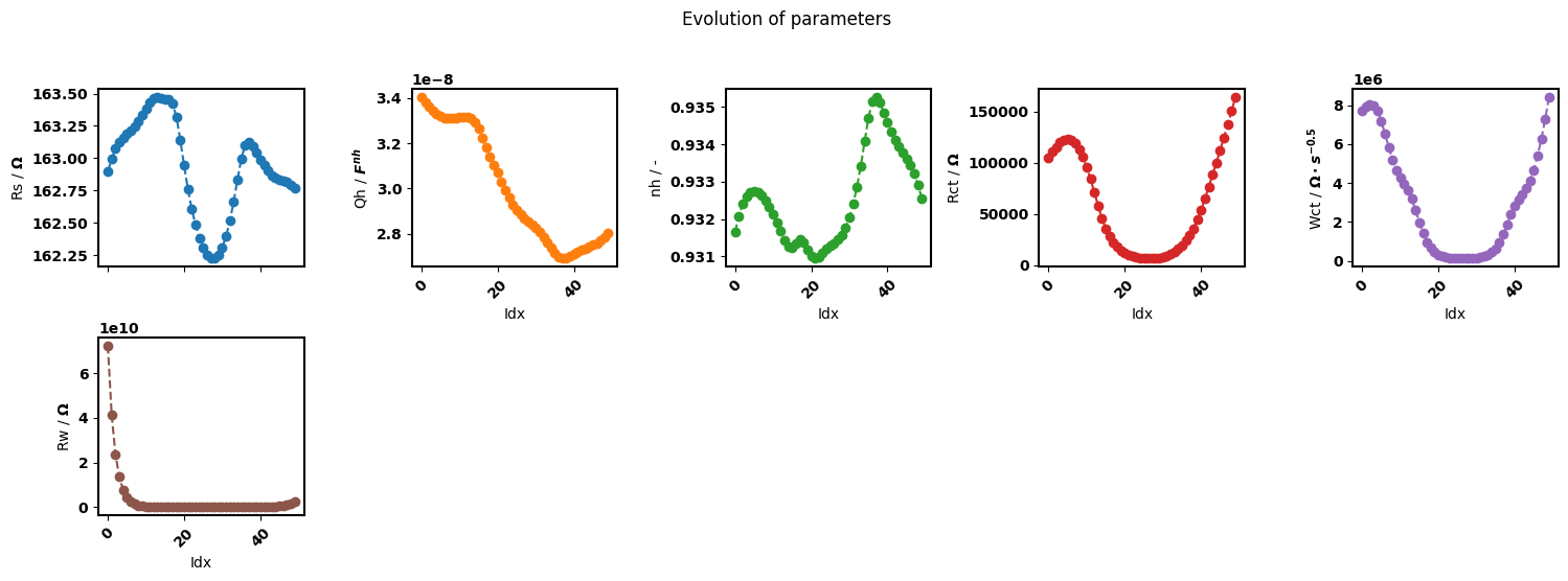
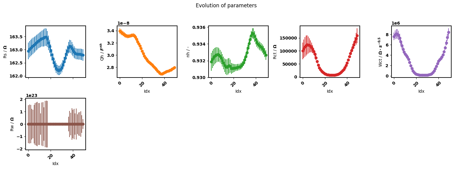
labels = {"Rs":"$\Omega$", "Qh":"$F^{nh}$", "nh":"-", "Rct":"$\Omega$", "Wct":"$\Omega\cdot s^{-0.5}$", "Rw":"$\Omega$"}
1. using the standard deviation as weighting
[8]:
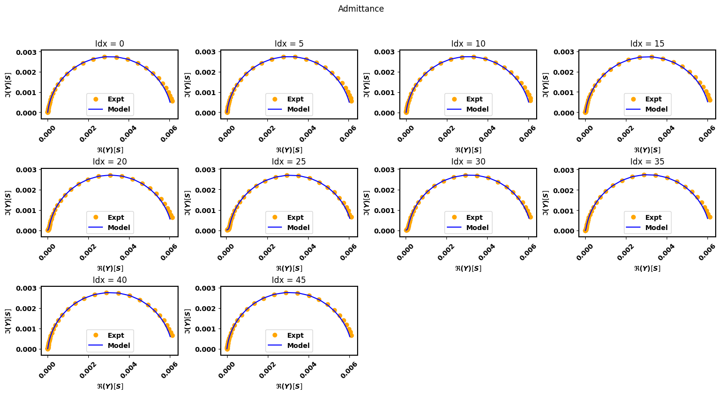
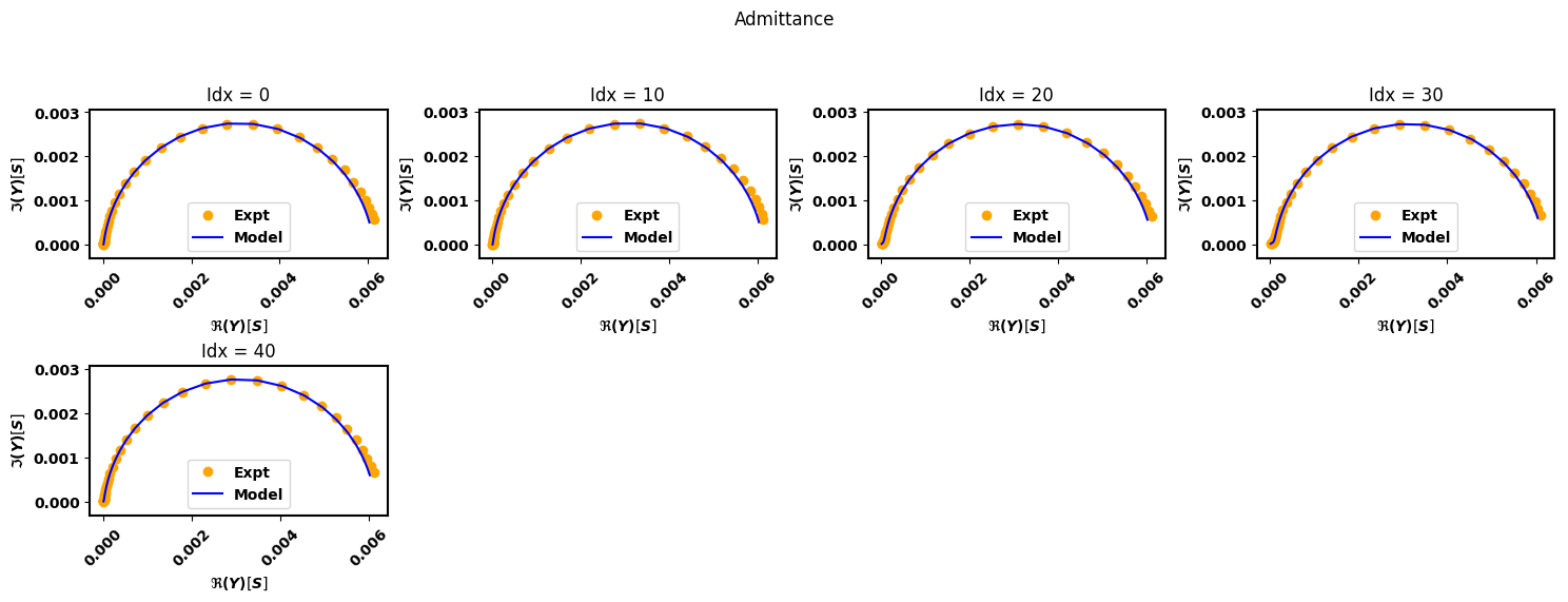
eis_redox_sigma = pym.Multieis(p0, F, Y, bounds, smf_sigma, redox, weight= Yerr, immittance='admittance')
[9]:
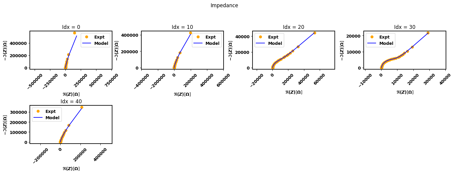
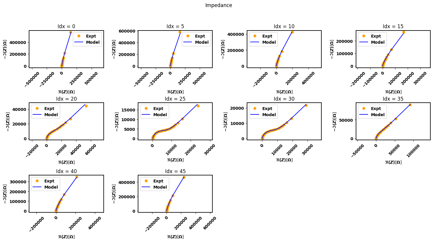
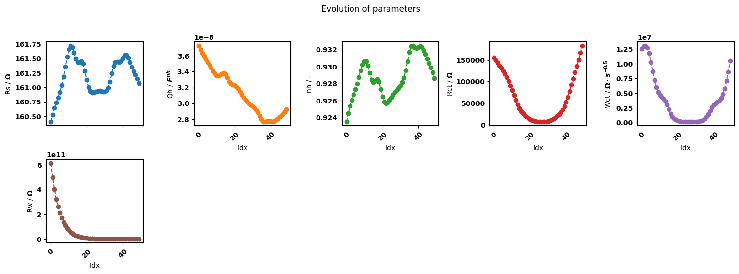
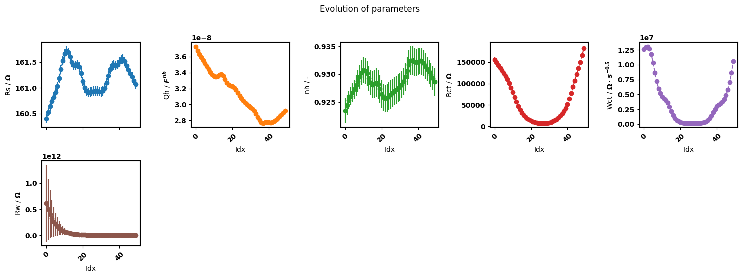
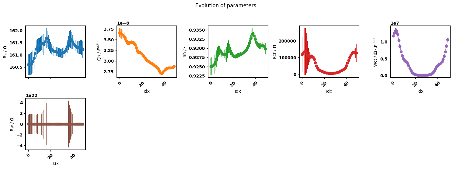
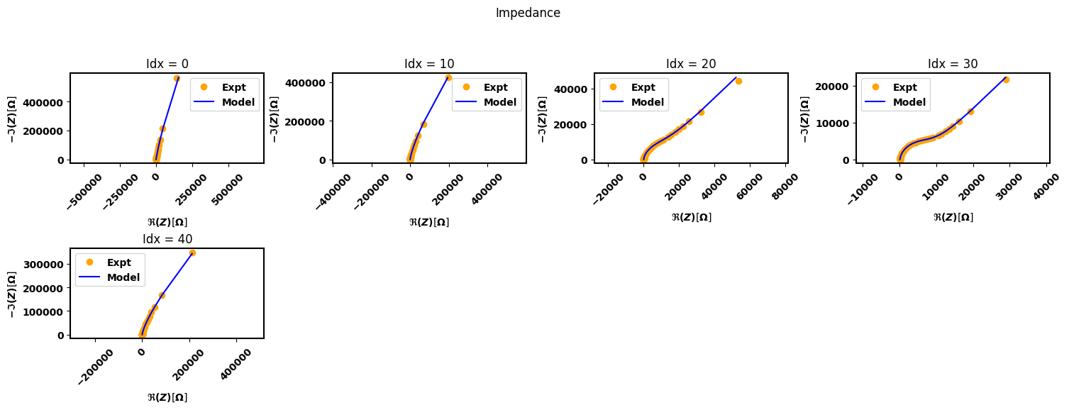
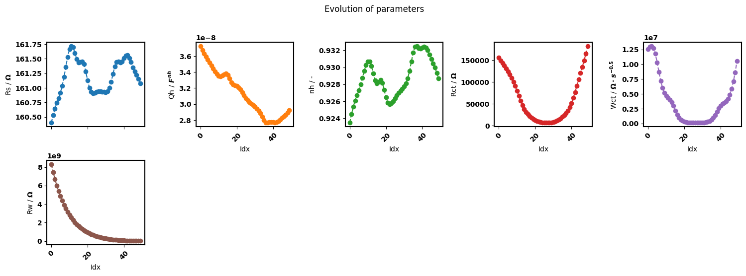
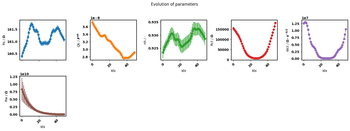
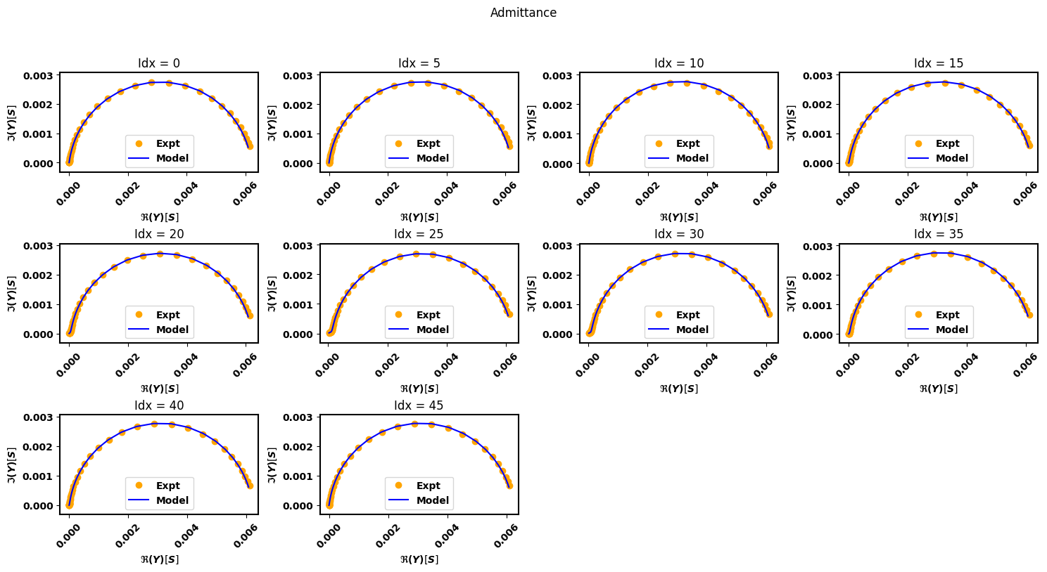
popt, perr, chisqr, chitot, AIC = eis_redox_sigma.fit_simultaneous(method = 'tnc')
eis_redox_sigma.plot_nyquist(5)
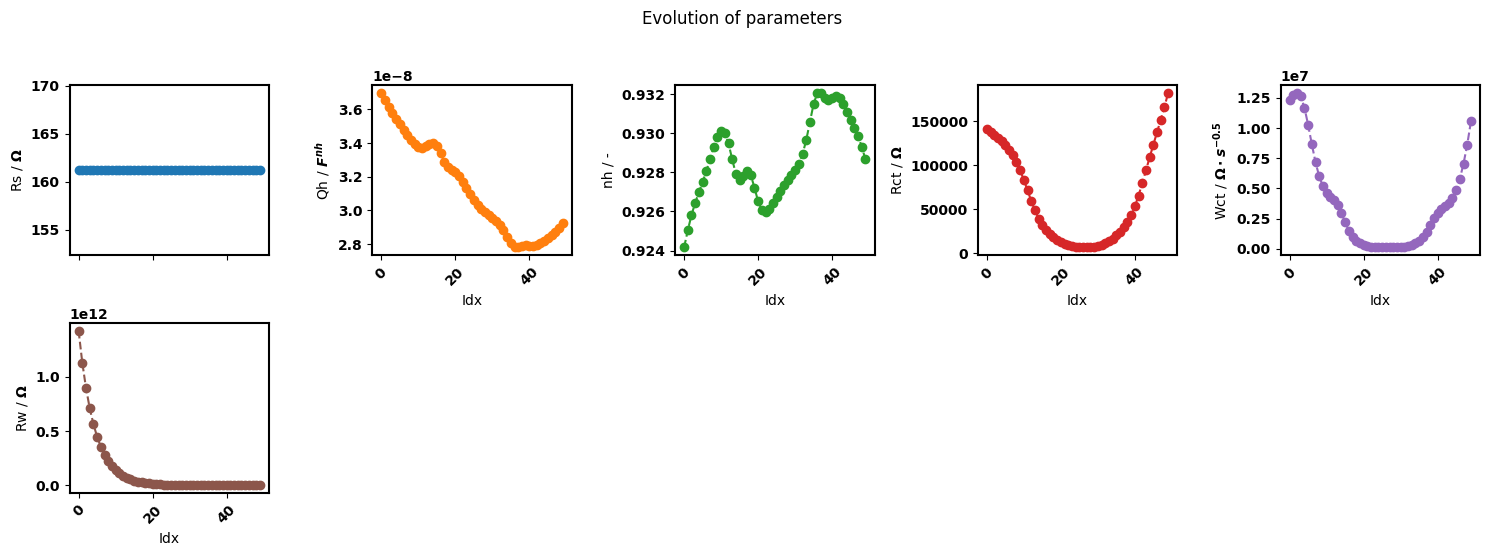
eis_redox_sigma.plot_params(labels=labels)
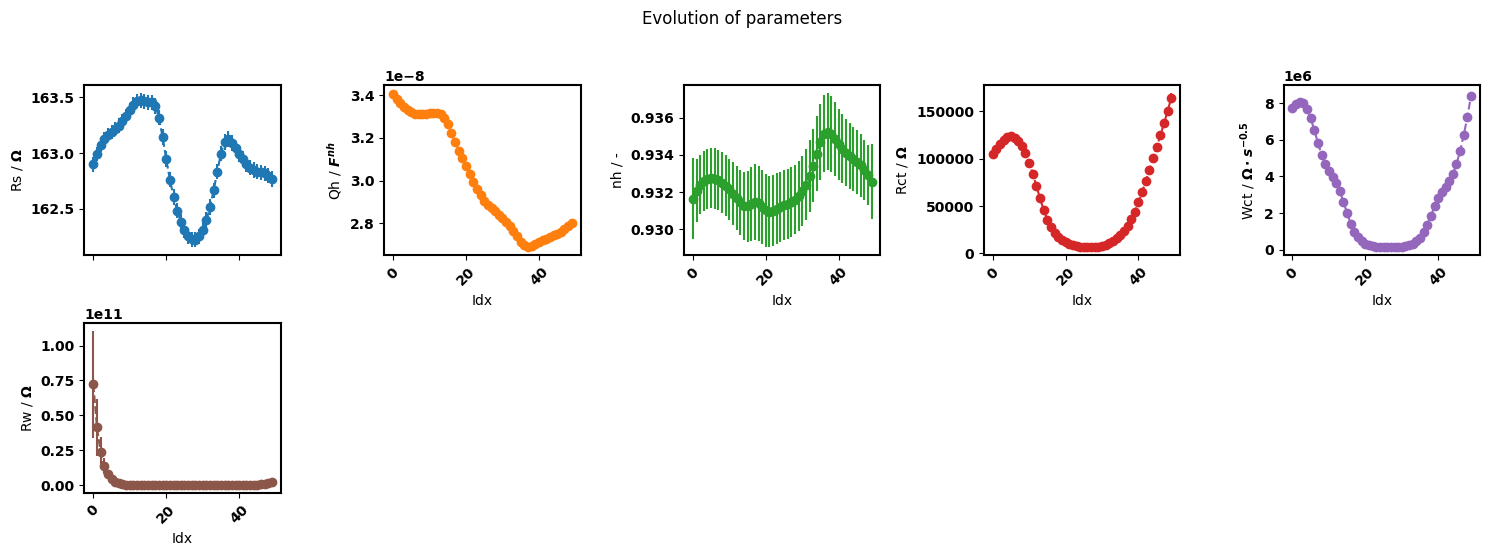
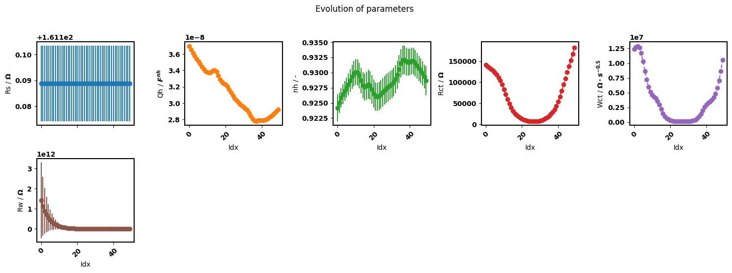
eis_redox_sigma.plot_params(True, labels=labels)
Using initial

Optimization complete
total time is 0:00:15.647183
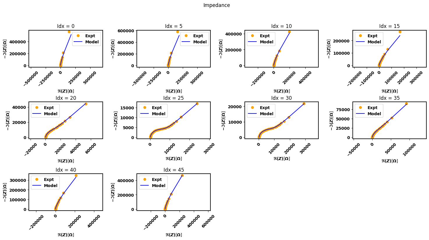
[10]:
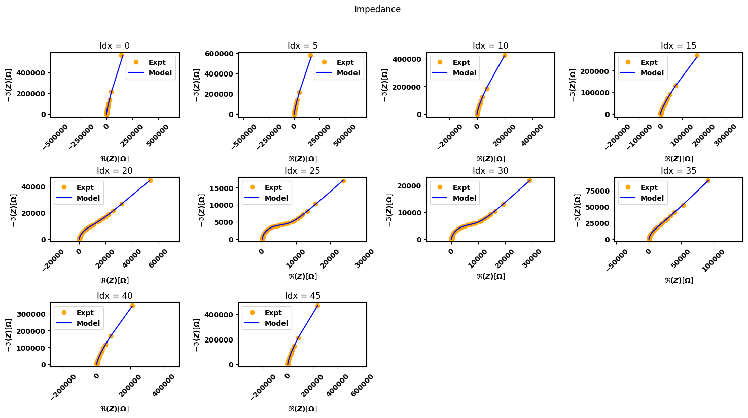
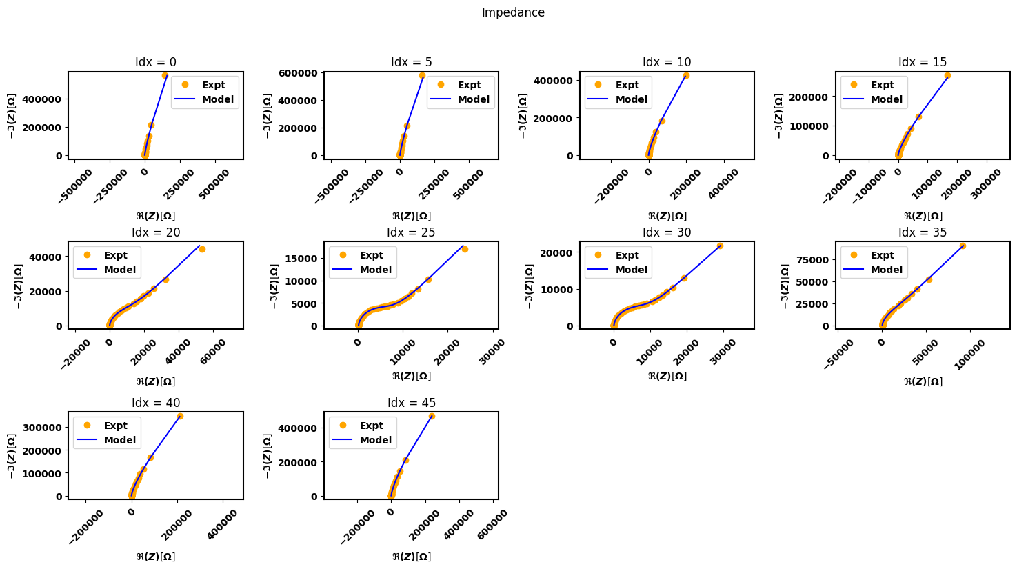
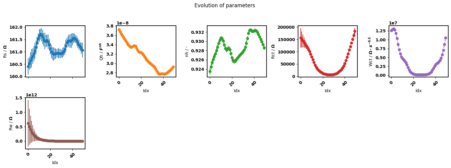
popt, perr, chisqr, chitot, AIC = eis_redox_sigma.fit_simultaneous_zero()
eis_redox_sigma.plot_nyquist(10)
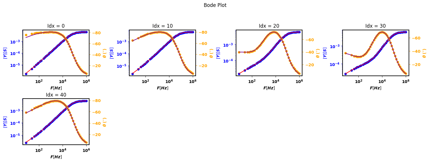
eis_redox_sigma.plot_bode(steps = 10)
eis_redox_sigma.plot_params(labels=labels)
eis_redox_sigma.plot_params(True, labels=labels)
Using prefit

Optimization complete
total time is 0:00:09.716980

2. Using the modulus as weighting
There are many cases where we do not have the data for the standard deviation of the admittance or impedance. pymultipleis offers other weighting options. In this second example we shall fit using the modulus as the weighting. All you need do is set the weight to the string “modulus”.
[7]:
eis_redox_modulus = pym.Multieis(p0, F, Y, bounds, smf_modulus, redox, weight= 'modulus', immittance='admittance')
popt, perr, chisqr, chitot, AIC = eis_redox_modulus.fit_simultaneous(method = 'tnc')
eis_redox_modulus.plot_nyquist(5)
eis_redox_modulus.plot_params(labels=labels)
eis_redox_modulus.plot_params(True, labels=labels)
Using initial

Optimization complete
total time is 0:00:12.533008

[8]:
print(chitot)
3.742554443579488e-05
[13]:
popt, perr, chisqr, chitot, AIC = eis_redox_modulus.fit_simultaneous_zero(method='bfgs')
eis_redox_modulus.plot_nyquist(5)
eis_redox_modulus.plot_params(labels=labels)
eis_redox_modulus.plot_params(True, labels=labels)
Using prefit

Optimization complete
total time is 0:00:13.526634


Make a least squares fit directly after running fit_simultaneous()
Here fit_sequential() uses the optimal parameters produced from fit_simultaneous() as initial guesses.
[14]:
# Reinstantiate class
eis_redox_modulus = pym.Multieis(p0, F, Y, bounds, smf_modulus, redox, weight= 'modulus', immittance='admittance')
popt, perr, chisqr, chitot, AIC = eis_redox_modulus.fit_simultaneous(method = 'tnc')
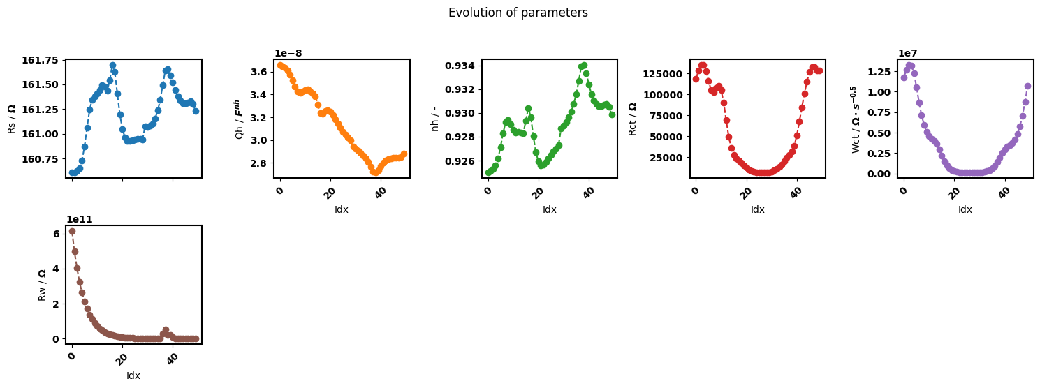
popt, perr, chisqr, chitot, AIC = eis_redox_modulus.fit_sequential(indices=None)
eis_redox_modulus.plot_nyquist(5)
eis_redox_modulus.plot_params(show_errorbar = False, labels = labels)
eis_redox_modulus.plot_params(show_errorbar = True, labels = labels)
Using initial

Optimization complete
total time is 0:00:07.181593
Using prefit
fitting spectra 0
fitting spectra 10
fitting spectra 20
fitting spectra 30
fitting spectra 40

Optimization complete
total time is 0:01:08.218272

3. Fitting with the stochastic option
[15]:
# Reinstantiate class and fit stochastic
eis_redox_modulus = pym.Multieis(p0, F, Y, bounds, smf_modulus, redox, weight= 'modulus', immittance='admittance')
popt, perr, chisqr, chitot, AIC = eis_redox_modulus.fit_stochastic()
eis_redox_modulus.plot_nyquist(10)
eis_redox_modulus.plot_params(show_errorbar = False, labels = labels)
eis_redox_modulus.plot_params(show_errorbar = True, labels = labels)
Using initial
0: loss=4.119e-01
10000: loss=4.565e-05
20000: loss=3.768e-05
30000: loss=3.753e-05
40000: loss=3.749e-05
50000: loss=3.748e-05
60000: loss=3.747e-05
70000: loss=3.746e-05
80000: loss=3.746e-05
90000: loss=3.745e-05
Optimization complete
total time is 0:01:51.632921

4. Running the Bootstrap MonteCarlo option
[16]:
# Reinstantiate class and fit stochastic
eis_redox_modulus = pym.Multieis(p0, F, Y, bounds, smf_modulus, redox, weight= 'modulus', immittance='admittance')
popt, perr, chisqr, chitot, AIC = eis_redox_modulus.fit_simultaneous(method = 'tnc')
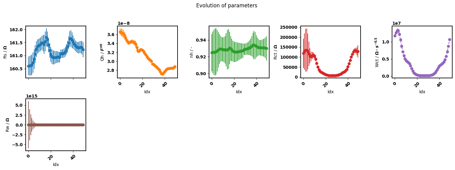
popt, perr, chisqr, chitot, AIC = eis_redox_modulus.compute_perr_mc(n_boots=500)
eis_redox_modulus.plot_nyquist(5)
eis_redox_modulus.plot_params(show_errorbar = False, labels = labels)
eis_redox_modulus.plot_params(show_errorbar = True, labels = labels)
Using initial

Optimization complete
total time is 0:00:07.882804
Please run fit_simultaneous() or fit_stochastic()
              on your data before running the compute_perr_mc() method.
              ignore this message if you did.

Optimization complete
total time is 0:43:47.656617


5. Keeping a parameter constant
[17]:
# Reinstantiate class and fit keeping a parameter constant
smf_const = smf_modulus.at[0].set(jnp.inf) # Here we use JAX's index update syntax to modify the element of smf_modulus
eis_redox_modulus = pym.Multieis(p0, F, Y, bounds, smf_const, redox, weight= 'modulus', immittance='admittance')
popt, perr, chisqr, chitot, AIC = eis_redox_modulus.fit_simultaneous(method = 'tnc')
eis_redox_modulus.plot_nyquist(5)
eis_redox_modulus.plot_params(show_errorbar = False, labels = labels)
eis_redox_modulus.plot_params(show_errorbar = True, labels = labels)
Using initial

Optimization complete
total time is 0:00:11.090526

6. Saving the plots
[18]:
eis_redox_modulus.save_plot_nyquist(steps=10, fname='example_results')
eis_redox_modulus.save_plot_bode(steps=10, fname='example_results')
eis_redox_modulus.save_plot_params(False, fname='example_results')
7. saving the results
[19]:
eis_redox_modulus.save_results(fname='example_results')